Preprint
Centrifugal compressor impeller blades with a Bernoulli lemniscate segment as the camber line
L. Artilakva · 2013
Analytical construction, polar parametrization, eleven reference points for a 560 mm impeller, and signed curvature compared with a circular arc.
DOI: 10.5281/zenodo.24083341
Abstract. This paper presents an analytical construction of a centrifugal compressor impeller blade camber line from a smooth Bernoulli lemniscate segment with centrally symmetric endpoints. The implicit curve equation yields an explicit expression for the ordinate that accounts for its sign on either side of the node. Formulas are derived for rotation to the specified inlet angle and uniform scaling using the intersection of the chord with the outlet circle. Expressions are obtained for the arc length, curvature and geometric outlet angle. The paper also specifies conditions under which the segment can be used for a radially extending blade and establishes the limits of aerodynamic interpretation of the geometry.
Keywords. Centrifugal compressor, impeller, blade camber line, Bernoulli lemniscate, curvature, blade design.
1. Introduction
In plan view, the camber line sets the blade direction between the leading and trailing edges. Together with the thickness distribution, flow-path width and arrangement of neighbouring blades, it determines the geometry of the blade passage. With fixed inlet and outlet diameters and the same edge angles, different camber lines can produce different tangent directions and flow areas inside the impeller. These differences influence where the flow turns, accelerates or decelerates along the passage and how the load is distributed over the blade surfaces.
In geometric blade design, the camber line can be specified as a circular arc, which has constant curvature. In aerodynamic design, the blade shape can be determined from a prescribed distribution of relative velocity over its surfaces [1, 2]. The geometric formulation considered here defines an analytical family of lines for which the tangent direction and curvature can be calculated along the entire segment between the edges. The initial geometry can therefore be assessed before the flow field is calculated.
The selected lemniscate segment passes through the node along one smooth branch. At the midpoint, the curvature reaches zero and changes sign. On either side of the inflection point, its magnitude increases with distance from the node. The tangent therefore turns along two joined segments with no discontinuity in direction or curvature. Central symmetry relates the end tangents. Once the curve is placed in the impeller, this relation must be consistent with the required edge positions and outlet angle.
1.1. Gas-dynamic basis for the choice of curve
When a relative streamline in the two-dimensional model is close to the blade camber line, the streamline’s geometric curvature enters the normal component of acceleration. For relative speed and signed streamline curvature , The curvature distribution of the camber line gives a geometric indication of how this acceleration varies. At the same , a smaller magnitude of streamline curvature corresponds to a smaller normal acceleration magnitude. For steady flow in a frame rotating at constant angular velocity , the normal projection of the momentum equation is Here is pressure, is gas density, is the viscous stress tensor, is the position vector relative to the rotation axis and is the left-hand unit normal to the planar streamline. The geometric contribution is considered together with the Coriolis and centrifugal forces. The curvature of the camber line alone does not determine the pressure distribution, boundary-layer development or the location of separation.
The analogy with a particle moving along a prescribed arc can be formulated for ideal frictionless motion in a potential field . Let be the particle’s initial speed and the distance along the path. The travel time along the arc is Equal travel times along the arc and chord would require the corresponding integrals to agree for the prescribed initial conditions and field. In an impeller, pressure and viscous stresses also affect the gas flow. The engineering case for selecting the lemniscate therefore rests on its calculable curvature distribution and on the ability to fit it to the impeller geometry. Reduced losses and higher efficiency remain hypotheses to be tested by gas-dynamic analysis.
2. Initial lemniscate branch
Let and be the diameters of the circles that locate the beginning and end of the camber line in the impeller plan view. In the local system , the lemniscate foci have coordinates and , where is the distance from the node to either focus. The parameter and the half-span of the selected segment along the axis are defined by Writing , the classical equation of the lemniscate is [3]. In the notation used here, it follows directly from the condition that the product of the distances to the foci is constant Define . Solving for gives In Figure 1, the branch passes from the third quadrant into the first. The signs of and therefore coincide. The sign of the ordinate matters. Using the same square-root sign on both sides of the node would join segments with different tangents.
The rationalized form is convenient for calculations near the node and shows that the branch extends analytically through it The function is odd. In the last formula, the expression under the square root is positive over the entire selected interval. The segment endpoints, chord and chord length are obtained in sequence
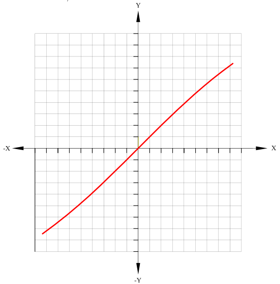
(a) Smooth branch in local coordinates
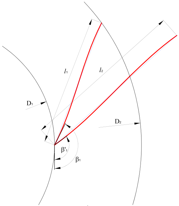
(b) Rotation and alignment with the circles
3. Tangent and curvature of the initial segment
For , differentiate the identity The tangent remains continuous at the node. Expanding the rationalized form gives The derivative is even, so . In local coordinates, the angle describes the inlet tangent direction. Its slope is the limit of the secant slopes The signed curvature is defined for traversal in the direction of increasing . For , the second derivative and curvature are Let be the distance to the node and the local polar angle. On the positive half of the branch, . Differentiating with respect to gives The last expression gives the curvature for increasing . On , the ratio decreases because the numerator under the square root in its rationalized form decreases while the denominator increases. Thus decreases as increases. Using the odd symmetry of and the even symmetry of , the resulting law over the entire segment is In particular, increases with . The curvature magnitude reaches its maximum at the ends of the chosen branch, and the inflection point is at the node.
4. Fitting the curve to the impeller
4.1. Aligning the inlet point and tangent
The origin of the global system is located on the impeller axis. The axis extends radially toward the inlet point . Positive rotation is counterclockwise. The geometric inlet angle is measured from the tangent opposite to rotation toward the outward radial direction. The radii and specified unit inlet tangent are The initial angle is measured from the same reference direction after translating the start of the segment to . The rotation angle is the difference between the two angles The entire segment is translated and rotated. In particular, the rotated chord is obtained from the difference between its original endpoints
4.2. Intersecting the ray with the outlet circle
A ray is drawn from in the direction of the rotated chord. Its intersection with the circle of radius is determined by the positive parameter satisfying Since , the quadratic has exactly one positive root. It gives the intersection in the direction from inlet to outlet. Setting yields For a line written as with , the intersection equation takes the scalar form Of the two intersections of the line and circle, choose the one satisfying . The vector form also applies to a vertical chord.
4.3. Final camber-line equation
Uniform scaling is carried out about the inlet point . Main equation for the blade camber line In the impeller coordinate system, The parametric form preserves the correspondence between points before and after the transformation. Uniform scaling of the local formula itself uses the identity The local interval becomes . Rotation aligns the inlet tangent with , and scaling preserves the aligned direction. By construction, , and .(57)
5. Checking the geometry and outlet angle
The transformed unit tangent to the impeller blade camber line, arc length and curvature are A positive scale factor preserves tangent directions and changes the arc length and curvature magnitude. In global coordinates, the inflection point is at the chord midpoint To check the radial progression, calculate the distance to the axis and its derivative For , a sufficient condition for the curve to be single-valued as a function of radius over the full interval is . This condition needs to be checked in addition to placing the endpoints on their circles. When , the radial and circumferential projections of the tangent at the local geometric angle give The circumferential position of the camber line therefore depends on the angle distribution along its full length.
Define radial and circumferential unit vectors at the outlet. The circumferential direction is the positive direction of rotation The geometric outlet angle is determined from the projections of the tangent The signs of the two projections determine the quadrant of the angle. The end tangents of the initial branch point in the same direction, so . If is the signed polar angle of relative to the axis, then Given , and , the outlet angle of the symmetric segment follows from the construction. Both angles and both edge positions can be specified independently only if they satisfy this relation. When comparing shapes with fixed endpoints and angles, this condition is checked before comparing curvatures.
6. Camber line and blade passage
Figure 2 illustrates how different camber lines change the shape of a blade passage. The NPF HKS line (Khimmash-Kompressor Service research and production company) is constructed from a lemniscate. The LPI line follows the Leningrad Polytechnic Institute design method, and denotes a circular arc. The diagram shows the geometric differences and provides a basis for comparative calculations.
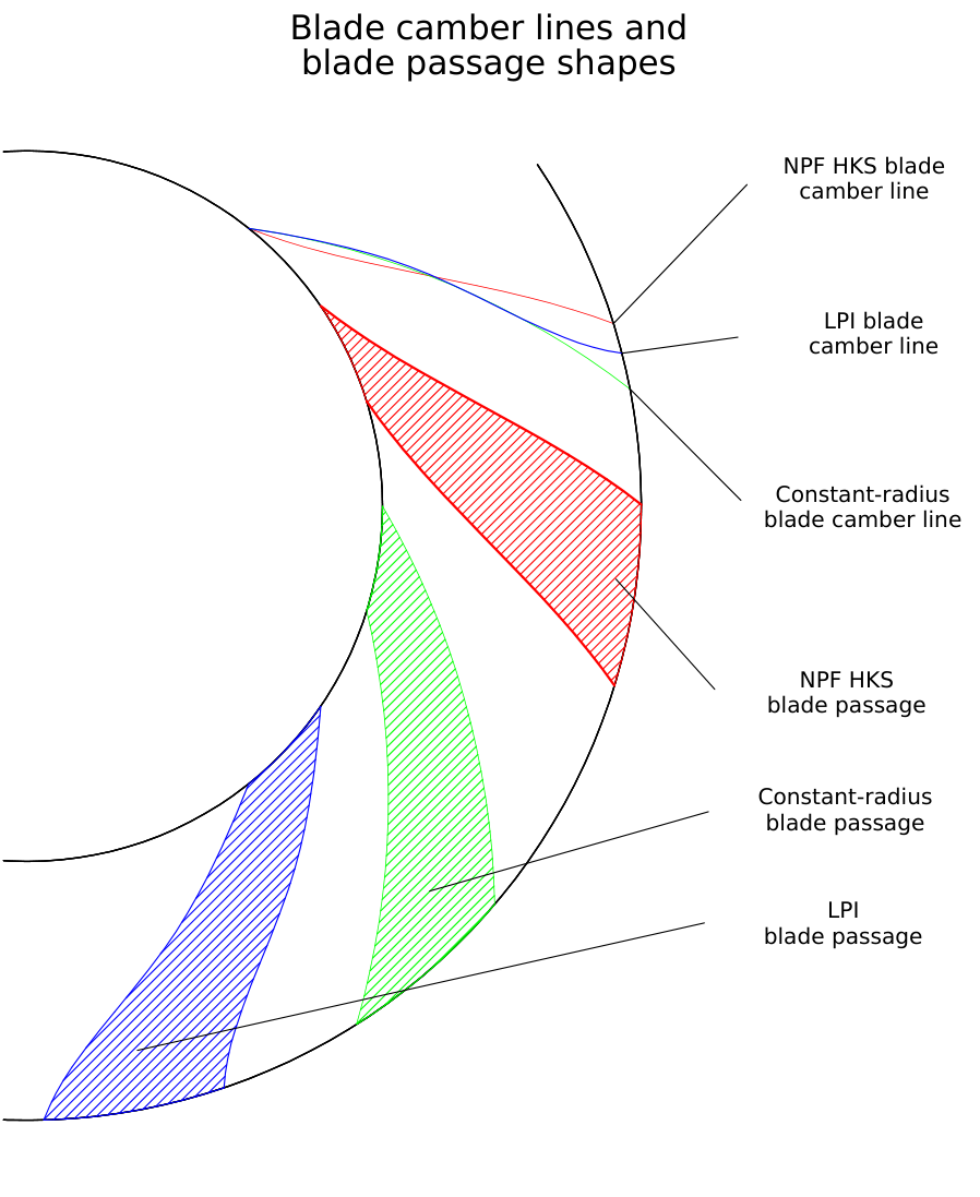
In the two-dimensional model, the blade sides are formed by applying the half-thickness distribution to the camber line. Let be the left-hand unit normal and the unit tangent. The two side curves are defined by The condition is sufficient for local regularity of both curves. Flow areas also depend on the impeller’s meridional width, thickness distribution and circumferential pitch. For a specified blade count , adjacent camber lines are obtained by rotating about the impeller axis through the angular pitch The geometric model is checked for flow areas, intersections between the sides of adjacent blades and agreement between the blade edges and meridional contours. To isolate the effect of curvature distribution in a comparative calculation, the edge positions, inlet and outlet angles, thickness distribution, meridional geometry, rotational speed, flow rate and inlet gas state are held fixed. Under these conditions, changes in the velocity field, losses and efficiency can be attributed to the camber-line shape within the accuracy of the calculation.
7. Conclusions
A symmetric segment of the Bernoulli lemniscate gives an analytically defined camber line with continuous tangent and curvature. Segments of opposite curvature meet at the inflection point. The curvature magnitude along each segment is determined by the distance to the node of the original curve and the scale factor.
The proposed construction aligns the inlet tangent with the specified geometric angle and places the outlet point on the outer circle. The positive scale factor is uniquely determined by the intersection of the rotated chord ray with that circle. The outlet angle follows from the relative positions of the endpoints and the fact that their tangents point in the same direction.
The gas-dynamic merits of this geometry can be assessed by examining the flow and losses in comparable passages. The expressions given here provide a reproducible starting geometry for that assessment.
8. Numerical example for the NPF HKS impeller
The diameters and specify the positions of the leading and trailing edges of the NPF HKS impeller blade. The calculation uses no intermediate rounding.
8.1. Initial lemniscate segment
8.2. Rotation and alignment with the outlet circle
8.3. Arc length and outlet angle
The camber-line length is calculated by integrating along the original branch and applying the scale factor. The tabulated geometric outlet angle for the NPF HKS impeller is . The absolute difference is
8.4. Polar parameterization and reference points
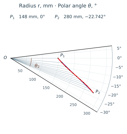
The pole is on the impeller axis. The ray passes through the leading edge . The polar angle is positive counterclockwise. In this example it is negative beyond the leading edge. The angle gives the position of a point, while gives the tangent inclination relative to the local circumferential direction.
Direct calculation of coordinates. Introduce a dimensionless parameter on the selected smooth branch. For , set equal to with the sign of matching the sign of . Substitution in the original lemniscate equation and continuation through the node give Here corresponds to the inlet, to the inflection point and to the outlet. In the global system, the centre of symmetry and the numerator of the position vector are The polar coordinates therefore follow directly from the parameter In general, the signs of both coordinates determine the quadrant. This form allows the entire curve to be plotted by direct substitution of values of . If the input is the angle , the radius is obtained algebraically from the intersection of a ray and the selected branch. Substitute the following expression in the original equation From the roots of the resulting quartic equation in , select the intersection with the required branch between and .
Uniform radial spacing. The table retains 11 reference points, including both blade edges. The radial conditions and coefficient definitions are Since , expanding gives For intermediate radii, select the real root on . The radius increases along this segment, so each has a unique root. The values in the table are obtained from the roots of the polynomial and the formula for .
| No. | , mm | , degrees |
|---|---|---|
| 1 | ||
| 2 | ||
| 3 | ||
| 4 | ||
| 5 | ||
| 6 | ||
| 7 | ||
| 8 | ||
| 9 | ||
| 10 | ||
| 11 |
8.5. Signed curvature distribution
For traversal from inlet to outlet, the curvature as a function of radius is given parametrically by The second formula follows from and the scaling of the curve. The curvature is zero at the inflection point . For this impeller, the calculation gives The circular arc passes through and with the same inlet tangent. With left-hand unit normal at the inlet and chord , equating the distances to the centre of the circle gives
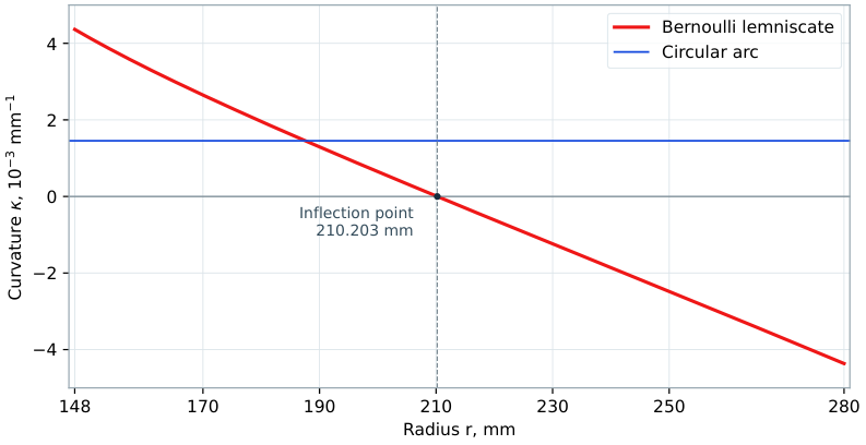
The lemniscate’s signed curvature decreases and changes sign. Its magnitude is smaller than that of the circular arc near the inflection point and larger at the edges. The outlet tangents differ. Comparing losses and efficiency requires a flow calculation under matched conditions.
References
- Jansen W., Kirschner A. M. Impeller Blade Design Method for Centrifugal Compressors. In: Fluid Mechanics, Acoustics, and Design of Turbomachinery, Pt. 2. 1974. NASA NTRS 19750003125.
- Aungier R. H. Centrifugal Compressors. A Strategy for Aerodynamic Design and Analysis. ASME Press, 2000.
- Lemniscate. Encyclopædia Britannica. 11th ed., 1911.