Research · 2014
Performance of centrifugal compressor impellers with LPI and NPF HKS blade camber lines
L. Artilakva
ANSYS 14.5 comparison at 8,000 rpm, including velocity triangles, two operating points and the construction of the HKS blade camber line from a Bernoulli lemniscate.
DOI: 10.5281/zenodo.24080443
Download the original Russian PDF ↓Impeller performance and operating conditions
LPI denotes a blade camber line constructed by the Leningrad Polytechnic Institute method. NPF HKS denotes a camber line constructed by the method of the Khimmash-Kompressor Service research and production company.
L. Artilakva. Comparison at 8,000 rpm and 126.7 kPa downstream of the diffuser.
Abstract. The study was carried out in 2014. Two blade shapes were compared using ANSYS 14.5 results. At the operating points examined, HKS delivered 23.6% more mass flow with 10.2% more power. Specific work calculated from power and flow fell by 10.85%. The hydraulic efficiency was 7.17 percentage points higher, and the polytropic efficiency calculated from the heads was 4.46 percentage points higher.
Operating conditions. The working fluid was air. Suction conditions were 101 kPa and 298 K. The analysis used cₚ = 1.006 kJ·kg⁻¹·K⁻¹ and k = 1.4. A density of 1.1455 kg·m⁻³ was used to convert mass flow to volumetric flow. Section 06 gives the pressure-ratio calculation.
Both impellers have 21 blades, an outside diameter of 0.560 m and an outlet width of 0.037 m. The diffuser diameters range from 0.560 to 0.880 m, and its width is 0.037 m. The inlet camber-line angle is 39.069° for both designs. The outlet angle is 61.829° for HKS and 72.642° for LPI.
Table 1. Flow, power and efficiency. The entries are HKS, LPI, and the HKS difference relative to LPI, respectively.
Volumetric flow from the source table, m³·h⁻¹ — 27,323 · 22,109 · +23.6%. Mass flow G, kg·h⁻¹ — 31,298 · 25,326 · +23.6%. Mass flow ṁ, kg·s⁻¹ — 8.694 · 7.035 · +23.6%.
Power N, kW — 213.548 · 193.829 · +10.2%. Specific work, kJ·kg⁻¹ — 24.56 · 27.55 · −10.85%. Hydraulic efficiency — 93.38% · 86.21% · +7.17 percentage points. Polytropic efficiency from the heads — 85.03% · 80.56% · +4.46 percentage points.
The source labels volumetric flow in normal cubic metres per hour. The figures were obtained by dividing G by the assumed density of 1.1455 kg·m⁻³. The source does not specify the reference conditions.
Data source. Results of the thermogasdynamic calculation of impellers with LPI and NPF HKS blade camber lines, ANSYS 14.5, lpi_xkc.1.pdf, pp. 1–2.
Stage flow — impeller and diffuser
Station 1 is the impeller inlet, 2 the impeller outlet, 3 the diffuser inlet and 4 the diffuser outlet. Pressure and temperature symbols follow the source table.
Table 2. Flow parameters and calculated heads. HKS values are given first, followed by LPI values.
Pressures P₁ and P₂, kPa — 89.9, 112.9 / 94.2, 114.5. Pressures P₃ and P₄, kPa — 114.0, 126.7 / 115.1, 126.7. Temperatures T₁ and T₂, K — 288.3, 311.2 / 292.1, 313.0. Temperatures T₃ and T₄, K — 311.0, 321.5 / 313.4, 323.2.
Absolute speed C₁ and C₂, m·s⁻¹ — 106.7, 183.2 / 106.3, 168.5. Relative speed in the radial–circumferential plane, m·s⁻¹ — 152.41, 120.18 / 141.02, 112.32. Radial velocity Cᵣ₁ and Cᵣ₂, m·s⁻¹ — 102.5, 92.6 / 98.0, 74.9. Circumferential velocity Cᵤ₁ and Cᵤ₂, m·s⁻¹ — 29.6, 158.0 / 41.0, 150.9. Blade speed U₁ and U₂, m·s⁻¹ — 142.4, 234.6 for both.
Flow coefficient φ₂ — 0.3947 / 0.3193. Relative outlet angle β₂ — 50.40° / 41.82°. Deviation angle from the velocity triangles — 11.43° / 30.82°.
Polytropic and isentropic heads, kJ·kg⁻¹ — 19.588, 19.476 / 16.939, 16.825. Internal head hᵢ, kJ·kg⁻¹ — 23.037 / 21.025. Dynamic head hD, kJ·kg⁻¹ — 11.089 / 8.546. Euler head hₑ, kJ·kg⁻¹ — 32.852 / 29.563. Tabulated total head hᵢ + hD, kJ·kg⁻¹ — 34.126 / 29.572.
Impeller. At the HKS outlet, radial velocity is 23.6% higher and circumferential velocity is 4.7% higher. Static pressure rises by 23.0 kPa in HKS and by 20.3 kPa in LPI. The HKS static pressure is 4.3 kPa lower immediately at the impeller inlet and 1.6 kPa lower at the impeller outlet.
Diffuser. Static pressure rises by 12.7 kPa with HKS and 11.6 kPa with LPI. The increase in dynamic head through the HKS impeller is also greater. Comparing diffuser losses requires total pressures at stations 3 and 4.
The angles in the table were reconstructed from averaged velocity components. Section 05 gives the numerical substitutions.
Geometry and ANSYS input data
The operating points have the same rotational speed and pressure downstream of the diffuser. The flow-field values come from the archived ANSYS 14.5 table. The analysis distinguishes quantities recoverable from the published values from those requiring exported flow fields or geometry.
Table 3. Dimensions and calculation settings. HKS values are given first where they differ from LPI.
Inlet diameter, hub diameter and D₁, m — 0.340, 0.156, 0.296 for both. D₂, D₃ and D₄, m — 0.560, 0.560, 0.880 for both. Widths b₁, b₂, b₃ and b₄, m — 0.0514, 0.037, 0.037, 0.037 for both. Blade count z — 21 for both.
Camber-line angles β₁ and β₂ — 39.069°, 61.829° / 39.069°, 72.642°. Mesh size and iteration count — 117.6 million, 150 / 94.5 million, 150. Mesh factors, including the blade passage factor — 1.5 and 3 for both. Final tabulated residual — 7 × 10⁻⁶ for both.
Impeller volume Vₖ, m³ — 0.0119704 / 0.0118533. Blade-passage volume Vₗ, m³ — 0.000570019 / 0.000564443. Blade surface area S, m² — 0.0152637 / 0.0145222. Static enthalpy loss ΔH, kJ — 0.0607534 / 0.10289.
The unit and figures for static enthalpy loss follow the source. The loss definition, normalization mass and control region are unspecified. An independent calculation requires all three. The source also leaves the type of final residual unspecified.
Geometric areas and volumes. Areas are in m², lengths in m and volumes in m³. Area A₂ was calculated before accounting for blade blockage. Independently checking blade area and impeller volume requires the original surfaces. The formulas use A for HKS and B for LPI.
Equations from the original study (p. 3)








Flow, power and specific work
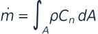
Mass and volumetric flow. Mass flow ṁ is expressed in kg·s⁻¹ and volumetric flow Q in m³·h⁻¹. The integral is taken over the control section, with Cₙ normal to that section.
Power and specific work. Torque M is expressed in N·m and was reconstructed on the assumption that N is impeller shaft power. The specific quantity q is expressed in W·h·kg⁻¹, and specific work l in kJ·kg⁻¹.
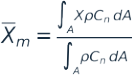
Averaging at a section. Pressures, temperatures and velocity components come from the ANSYS fields. The formula gives mass-flow weighting. Reproducing it requires the cell values and confirmation of the averaging convention used.
Equations from the original study (p. 4)















Velocity triangles
Blade speed, m·s⁻¹. The velocity triangles use the rounded blade speeds U₁ = 142.4 and U₂ = 234.6 m·s⁻¹. U₁ refers to the 0.340 m inlet diameter.
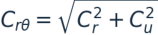
Absolute and relative velocity projections, m·s⁻¹. The projections are reconstructed from the averaged components. The dynamic head calculation instead uses the absolute velocity magnitudes from the computed field.
Flow and theoretical head coefficients are calculated from the velocity components and blade speeds shown in the equations.
Equations from the original study (p. 5)



















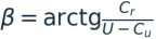
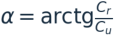
Flow angles
Angles reconstructed from the averaged velocity components.
The deviation angle δ is the difference between the blade camber-line angle and the reconstructed relative flow angle. All reconstructed angles refer to triangles based on averaged velocity components.
Equations from the original study (p. 6)








Static pressure and compression heads
Pressure differences in kPa and pressure ratios.
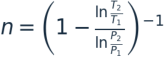
The polytropic exponent is determined from the pressures and temperatures at stations 1 and 2.
Polytropic and isentropic heads are expressed in kJ·kg⁻¹. The verification calculation uses R = 0.287 kJ·kg⁻¹·K⁻¹ and k = 1.4.
Equations from the original study (p. 7)
















Head and efficiency calculations
Energy balance. The calculations give the internal, Euler and dynamic heads in kJ·kg⁻¹, the total head in kJ·kg⁻¹, and the degree of reaction.
Hydraulic efficiency and polytropic efficiency calculated from the head ratio.
The same calculation is applied to both impellers in each pair. Efficiency differences are computed before rounding the individual values.
Equations from the original study (p. 8)

















Impeller outlet geometry and kinematics
The inlet camber-line angle is 39.069° for both designs, and the inlet diameters are identical. At the outlet, the camber-line angle is measured from the tangent opposite to rotation toward the radial direction. With this convention, 90° is radial. The HKS camber line at 61.829° is therefore more backswept, while LPI at 72.642° is closer to radial.
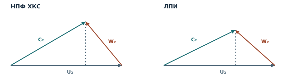
Figure 1 shows the triangles from the averaged velocity components at station 2. HKS has a 23.6% higher radial component and a 4.7% higher circumferential component. The geometric angle is compared with the relative angle β₂. The absolute angle α₂ describes the inlet conditions for the stationary diffuser.
Figure 1. Outlet velocity triangles on the same scale. The horizontal axis is the circumferential component in the direction of rotation, and the vertical axis is the outward radial component. The vectors close as C₂ = U₂ + W₂. The projection is onto the radial–circumferential plane.
Outlet deviation and geometric reference. If flow exited along the camber line, the calculated circumferential component would be greater for LPI. The actual ordering is reversed. Each impeller is evaluated at its own mass flow. Differences of 27.01 and 60.29 m·s⁻¹ measure the kinematic departure from that geometric reference.
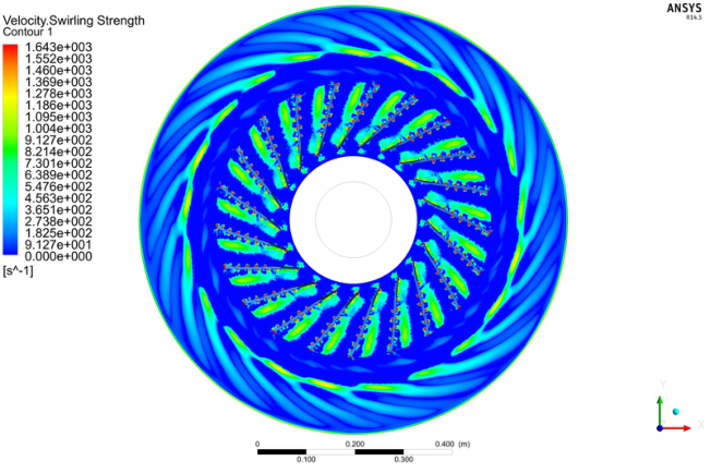
The smaller HKS deviation is consistent with the averaged outlet flow following the camber line more closely. The angle alone does not determine the extent of flow separation. Figure 6 shows local rotation using the Swirling Strength criterion. Comparable near-wall velocity and wall shear stress fields for both impellers are needed to assess separation and recirculation.
The local-rotation criterion is described by Zhou J., Adrian R. J., Balachandar S. and Kendall T. M., Journal of Fluid Mechanics, 1999, 387, 353–396. DOI 10.1017/S002211209900467X.
Equations from the original study (p. 9)






From swirl to head
The difference in Euler head has two nearly equal contributions. HKS has stronger outlet swirl and weaker inlet swirl in the direction of rotation. The calculation subtracts LPI from HKS and expresses the difference in kJ·kg⁻¹.
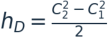
Decomposition of Euler head. The outlet absolute speed magnitudes give HKS a higher kinetic energy at station 2. In this article, the dynamic head hD expresses the increase in kinetic energy from station 1 to station 2. That increase accounts for 32.5% of hᵢ + hD for HKS and 28.9% for LPI.
Kinetic energy at station 2, kJ·kg⁻¹, and its share of the adopted impeller energy balance.
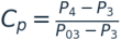
Diffuser static pressure increases by 12.7 kPa with HKS and 11.6 kPa with LPI. The final pressure is identical, and HKS has a 1.1 kPa lower static pressure at station 3. These values give the static pressure rise. To assess pressure-recovery performance and loss, normalization by the diffuser’s own inlet dynamic pressure is required.
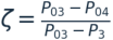
In the total-pressure coefficients, P₀₃ and P₀₄ denote total pressures at stations 3 and 4. Both variants require the same averaging convention. Substituting the impeller’s hD in the denominator would mix quantities from different sections. The available data cannot establish which diffuser has the lower total-pressure loss.
Equations from the original study (p. 10)







Effect of the camber line at the same flow rate
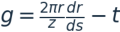
Eighteen vector points on the LPI camber line were extracted from Drawing 2 in the lemniscate paper. The radial coordinate was mapped onto the 148–280 mm interval. A cubic polynomial was used to adjust the interpolated circumferential coordinate so that both endpoint values and first derivatives matched the reconstructed HKS line. The two interpolation schemes used were a cubic spline and a shape-preserving piecewise cubic interpolant. The resulting LPI geometry was adapted for this comparison and differs from the original ANSYS model.
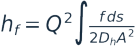
Both variants use inlet and outlet angles of 39.069° and 61.811°, a mass flow of 8.694 kg·s⁻¹ and 21 blades. Shared assumptions are a linear reduction in passage width from 51.4 to 37.0 mm, a constant blade thickness of 3 mm, a density of 1.1455 kg·m⁻³ and a Darcy friction factor of 0.020.
In the one-dimensional friction estimate, g is the approximate gap between blades, A the combined flow area, b the passage width, t the thickness, z the blade count, s the camber-line length, Dₕ the hydraulic diameter and Q the volumetric flow used in the model.
Table 4. Estimate with matching endpoints and tangents. HKS and drawing-based LPI camber-line lengths are 154.688 mm and 154.745–154.747 mm. The minimum computed flow area is 268.86 cm² for both. Specific friction loss is 1.048 kJ·kg⁻¹ for HKS and 1.084–1.090 kJ·kg⁻¹ for LPI.
Under these assumptions, estimated friction loss is 3.3–3.8% lower for the lemniscate, equivalent to 36–42 J·kg⁻¹. The minimum flow areas coincide. The integrated estimate depends on the changes in area, hydraulic diameter and velocity along the entire passage. The model does not resolve secondary flows, separation or mixing loss. The percentage describes estimated friction and cannot be converted directly into a stage efficiency gain.
Sources. L. Artilakva, Centrifugal compressor impeller with a blade camber line in the form of a Bernoulli lemniscate segment, 2024, Drawing 2. The one-dimensional formulas appear in the comparative calculation of the camber lines.
Equations from the original study (p. 11)


Impeller comparison — conclusions
Geometry. The HKS camber line is based on a Bernoulli lemniscate segment. A rotation of −86.25286° sets the blade’s geometric inlet angle to 39.069°. Uniform scaling by 0.6171998 brings the endpoint to the outer circle of radius 280 mm. The reconstructed outlet angle of 61.811° differs from the source value of 61.829° by 0.018°. The agreement applies to the outlet angle. The proximity of arc length (154.688 mm) to chord length (154.492 mm) is insufficient to establish the pressure distribution.
Original operating points. At 8,000 rpm and the same 126.7 kPa static pressure downstream of the diffuser, HKS has 23.6% more mass flow (8.694 versus 7.035 kg·s⁻¹) and 10.85% lower specific work calculated from power and flow (24.56 versus 27.55 kJ·kg⁻¹). The HKS Euler head is 3.29 kJ·kg⁻¹ higher. Stronger outlet swirl contributes 1.67 kJ·kg⁻¹ and weaker co-rotating inlet swirl contributes 1.62 kJ·kg⁻¹.
Kinematics. The deviation of relative flow from the camber line reconstructed from averaged velocity components is 11.43° for HKS and 30.82° for LPI. These angles describe the outlet direction. Assessing the extent of separation requires comparable near-wall fields. The polytropic exponents of 1.50495 and 1.54826 describe the pressure–temperature relationship between stations 1 and 2. Separate estimates of friction and heat transfer require additional data.
Efficiency and energy balance. By the definitions adopted here, HKS has a 7.17 percentage point advantage in hydraulic efficiency and a 4.46 percentage point advantage in polytropic efficiency calculated from the heads between impeller stations. Stage efficiency requires consistent total quantities upstream of the impeller and downstream of the diffuser. The discrepancy between specific work calculated from power and the rise in total enthalpy calls for checking torque, control-volume boundaries, and signed mass and energy fluxes.
Effect of camber-line shape. With matching endpoints, tangents and flow, the one-dimensional estimate gives HKS 3.3–3.8% less friction loss than the LPI line adapted from the drawing. The gain at the original operating points and the friction estimate with matched geometry describe separate comparisons. Paired three-dimensional simulations at identical flows can determine how curvature distribution contributes to stage efficiency. Industrial application also requires test-rig validation.
The HKS camber-line appendix gives the geometric construction, drawing and coordinate table.
Appendix — archived blade-passage flow maps
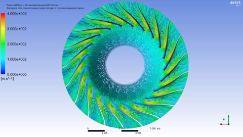
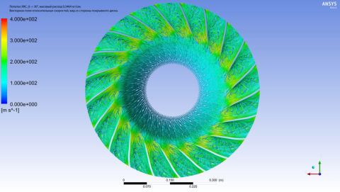
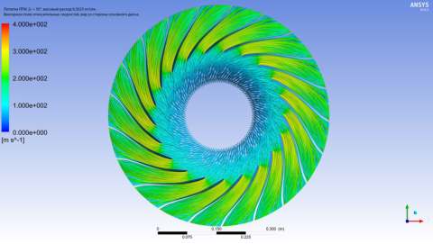
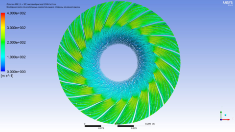
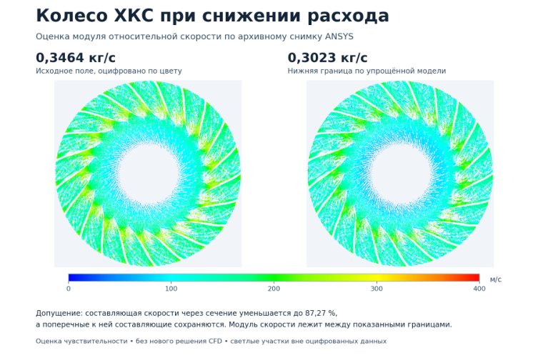
The labelled maps give 0.3023 kg·s⁻¹ for LPI and 0.3464 kg·s⁻¹ for HKS. Their correspondence to the operating points in Tables 1–3 has not been established. The maps show the flow structure at the conditions captured in the archive.
Figure 2. LPI on the left and HKS on the right, viewed from the shroud. The relative speed scale is 0–400 m·s⁻¹.
Figure 3. LPI on the left and HKS on the right, viewed from the hub disc, at the same flow rates and on the same scale.
On the shroud side, LPI has a more pronounced colour contrast across one blade pitch. Quantitatively comparing nonuniformity at the diffuser inlet requires radial velocity and absolute flow-angle fields over the full height of the same section.
Appendix — flow downstream of the impeller
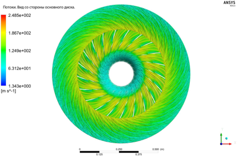
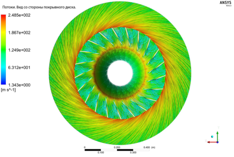
Figure 4. Streamlines viewed from the hub disc and shroud. The velocity scale is 1.343–248.5 m·s⁻¹.
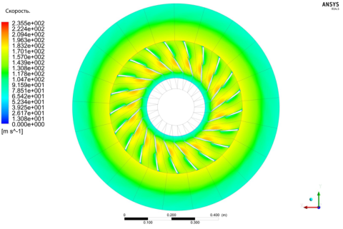
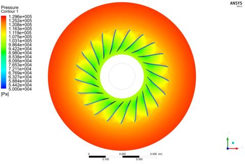
Figure 5. Maps of speed magnitude and static pressure. The scales are 0–235.5 m·s⁻¹ and 50–129.6 kPa. The archive does not establish the blade profile, flow rate, section heights or velocity reference frame for these maps.
In the outer annular region of Figure 5, the colour scales show falling speed and rising static pressure. Radial readings from a previous revision were about 160 to 85 m·s⁻¹ and 118 to 125 kPa between radii of 0.306 and 0.416 m. The values were read from separate maps and describe each individually.
On the original image scale, 990 pixels correspond to 0.400 m. The separate calculations estimate the annulus diameters, speed decrease and pressure increase.
Equations from the original study (p. 14)




Appendix — vortical regions and speed estimation
Figure 6. Swirling Strength, 0–1,643 s⁻¹. The map highlights regions of local flow rotation.
Figure 7. HKS viewed from the shroud. Left, the digitized map at 0.3464 kg·s⁻¹. Right, the lower bound of the estimated field at 0.3023 kg·s⁻¹. For this estimate, one velocity component was scaled and the other two were held constant. The result is an approximation from the archived visualization.
Equations from the original study (p. 15)

Appendix — construction of the NPF HKS blade camber line
Geometric reconstruction from a Bernoulli lemniscate segment.
Input data. The diameter at the start of the blade is D₁ = 296 mm. The outer impeller diameter is D₂ = 560 mm. The inlet angle is β₁ = 39.069°. Angles are measured from the tangent opposite to rotation toward the radial direction. The axis of rotation passes through the global origin O. Counterclockwise rotation is positive.
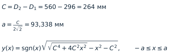
1. Select the lemniscate segment. C = D₂ − D₁ = 560 − 296 = 264 mm, and a = C/(2√2) = 93.338 mm. The sign of the ordinate follows Drawing 1 in the original work. The inlet and outlet points of the initial segment are symmetric about the local origin. Their ordinates are −83.378 and +83.378 mm.
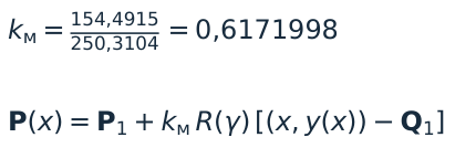
2. Align the inlet point and tangent. The segment’s inlet Q₁ is placed at P₁ = (148, 0) mm. The rotation is the difference between the required and initial tangent directions relative to the global X axis. The resulting rotation is γ = (39.069° − 90°) − 35.32186° = −86.25286°.
3. Extend the outlet to the outer circle. Draw a ray from P₁ along the rotated chord to the circle of radius r₂ = 280 mm. Scale the curve uniformly about P₁. The scale factor kₘ = 154.4915/250.3104 = 0.6171998. R(γ) is the planar rotation matrix for angle γ.
Equations from the original study (p. 16)

Appendix — reconstructed geometry and coordinates
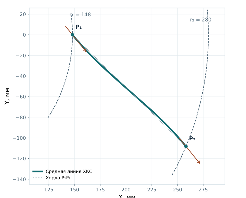
Plan view of the impeller. Coordinates are in millimetres, with equal scales on both axes. The plot shows the HKS camber line and chord P₁P₂, with radii r₁ = 148 mm and r₂ = 280 mm.
Reference coordinates. The parameter t runs from inlet (0) to outlet (1). Each entry gives t, X, Y and r, in that order. X, Y and r are in mm.
0.00 | 148.000 | 0.000 | 148.000 · 0.10 | 157.421 | −10.929 | 157.800 · 0.20 | 167.823 | −21.794 | 169.232 · 0.30 | 179.062 | −32.605 | 182.006.
0.40 | 190.923 | −43.374 | 195.787 · 0.50 | 203.115 | −54.122 | 210.203 · 0.60 | 215.308 | −64.870 | 224.868 · 0.70 | 227.169 | −75.639 | 239.431.
0.80 | 238.408 | −86.450 | 253.598 · 0.90 | 248.810 | −97.315 | 267.164 · 1.00 | 258.231 | −108.244 | 280.000.
Chord 154.492 mm. Arc length 154.688 mm. Reconstructed outlet angle 61.811°. The source table gives β₂ = 61.829°, an absolute difference of 0.018°.
Sources. L. Artilakva, Centrifugal compressor impeller with a blade camber line in the form of a Bernoulli lemniscate segment, 2024, pp. 5–9. Dimensions and angles are from the original LPI and NPF HKS calculation table (lpi_xkc.1.pdf).